Volume 17, Issue 1, January 2020
Computational Normative Decision Support Structures of Forensic Interpretation in the Legal Process
Alex Biedermann,* Silvia Bozza,** Franco Taroni,† and Joëlle Vuille‡
![]()
© 2020 Alex Biedermann, Silvia Bozza, Franco Taroni, and Joëlle Vuille
Licensed under a Creative Commons Attribution-NonCommercial-NoDerivatives 4.0 International License
Abstract
A broad range of questions at various instances in the legal process can be stated and analysed in terms of formal decision theoretic models, with results conveyed in graphical terms, such as decision trees. However, the real-world decision problems encountered by the participants of a legal process, including judges, prosecutors and attorneys, present challenging features, such as multiple competing propositions, variable costs and uncertain process outcomes. This complicates decision theoretic computations and the use of diagrammatic devices such as decision trees which mainly provide static views of selected features of a given problem. Yet, the issues are inherently dynamic, and the complexity of strategic planning and assessing legal tactics – given a party’s standpoint – increases even further when considerations are extended to information provided by forensic science services. This is because introducing results of forensic examinations may impact on the probability of various trial outcomes and hence crucially impact on a party’s interests. In this paper, we analyse and discuss examples of decision problems at the interface of the law and forensic science using influence diagrams (i.e., Bayesian decision networks). Such models, hereafter called normative decision support structures, can be operationally implemented through commercially and academically available software systems. These normative decision support structures represent core computational models that can be integrated as part of decision and litigation support systems, to help the participants of a legal process answer a variety of questions regarding complex strategic decisions.
Keywords
Decision theory, forensic science, dispute resolution, legal negotiation, Bayesian decision networks, normative decision policies, sequential decisions
Cite as: Alex Biedermann, Silvia Bozza, Franco Taroni, and Joëlle Vuille, "Computational Normative Decision Support Structures of Forensic Interpretation in the Legal Process" (2020) 17:1 SCRIPTed 83 https://script-ed.org/?p=3802
DOI: 10.2966/scrip.170120.83
* Faculty of Law, Criminal Justice and Public Administration, School of Criminal Justice, University of Lausanne, Lausanne, Switzerland, alex.biedermann@unil.ch
** Department of Economics, Ca’ Foscari University of Venice, Venice, Italy, silvia.bozza@unive.it ; Faculty of Law, Criminal Justice and Public Administration, School of Criminal Justice, University of Lausanne, Lausanne, Switzerland, silvia.bozza@unil.ch
† Faculty of Law, Criminal Justice and Public Administration, School of Criminal Justice, University of Lausanne, Lausanne, Switzerland, franco.taroni@unil.ch
‡ Faculty of Law, University of Fribourg, Fribourg, Switzerland, joelle.vuille@unifr.ch
1 Introduction
In light of the ever-increasing intricacy of legal practices, sound methodology to support thinking and making decisions in practical cases is a topic of interest for both researchers and practitioners. The central aspects of a given civil or criminal case, in particular those over which disagreement exists, need to be thought about in a structured way to enable insight and improve communication between various participants in the legal process. This includes lawyer and client relationships as well as the relationship between adversarial parties at trial. Methodologies for analysing legal cases, and their implementation, are pivotal topics for both practitioners and academics, because of the need to cope coherently with the problem of decision-making under uncertainty. For example, a party may need to decide whether to settle or plead guilty, whether to go to trial or how to allocate resources (e.g., to the search of further information). Such decisions place a party’s wealth, welfare or personal liberty at stake, and attorneys must thus formulate legal tactics that appropriately reflect the party’s preferences for or aversion to process outcomes. In litigation law, for example, factors such as the costs of going to trial, and the uncertainties about possible outcomes (verdicts) all need to be dealt with in a coherent whole. Such questions involve all the ingredients of classic decision theory: feasible decisions, uncertain states of nature, consequences (i.e., combinations of decisions and states of nature) and a valuation of the desirability (or, worth) of consequences. [1] Decision theory is strongly rooted in economics[2] and, following developments by several leading business school groups in the middle of the last century, it has also stimulated interest in the legal arena.[3] This interest has steadily increased and has been further strengthened, mainly since the 1980s, by the development of widely available computer systems capable of processing the mathematical form of legal decision models.[4] Such systems are not intended to replace various decision-makers in the legal process nor do such concepts claim to offer a comprehensive descriptive account of the various aspects of the legal process that they seek to model. Instead, such systems should best be considered as decision support devices to assist in the analysis of selected aspects of the densely connected network of factors upon which the outcomes of a case depend, at the level of detail that the user considers appropriate. Thus, they offer a normative perspective in the sense further discussed below.
The prototypical questions that have attracted wide interest among decision-theoretic researchers and legal scholars relate to the conviction or acquittal of defendants in the criminal trial, and the determination of the liability of defendants in civil lawsuits. These are important but far end points of legal processes. Decision theory, however, is a general theory for analysing how an individual, facing the question of what decision to make in situations of uncertainty, should proceed so as to insure coherence with that person’s judgments and preferences among possible decision outcomes.[5] In this paper, we build on existing works on decision theory for strategic questions arising in the legal context and then develop two extensions. The first is a translation of the standard model of legal negotiations, commonly represented in terms of decision trees,[6] into Bayesian decision networks, also sometimes called influence diagrams.[7] Bayesian decision networks are a highly flexible modelling environment that can be implemented using academically and commercially available software systems. The second extension concerns results of forensic examinations that may have an impact on trial outcomes, or intermediate steps in the legal process. To operate this second extension, we will take advantage of the fact that the use of graphical models, such as Bayesian networks and Bayesian decision networks, is already a well-established area of research for analysing the probative strength of forensic science results.[8] Thus, the question of how to logically connect reasoning models for legal negotiations and forensic results is an area which offers much room for fundamental research.
By choosing decision-theoretic graphical models we emphasise that the analyses pursued in this paper are normative,[9] i.e. focusing on explicit reference points against which one can compare one’s reasoning and conclusions in practical situations that require a decision to be made.[10] Stated otherwise, we will not deal with the empirical question of whether people’s actual behaviour conforms to the normative account of decision-making. There is, in fact, substantial evidence that people’s intuitive and unaided reasoning generally diverges from normative standards.[11] While descriptive research is important to assess the extent to which people think and act coherently, we maintain that this can only be achieved if the normative standpoints are first clarified (against which observable behaviour can be compared), and this is what the normative decision-theoretic structures developed throughout this paper seek to achieve. We will call our models computational normative decision support structures because our analyses, using formal approaches, focus on the conceptual relationship between traditional interpretation of forensic science results and strategic analysis in legal proceedings.
The paper is organized as follows. Section 2 briefly introduces the graphical models for decision-theoretic analyses used in later parts of the paper, i.e. decision trees and Bayesian decision networks (influence diagrams), using a general example of plea bargaining from the defendant’s point of view. Readers well acquainted with these concepts may skip this section. Section 3 starts with an outline of how to state the general model of legal negotiations in terms of a Bayesian decision network. Extensions regarding litigation costs, uncertainty factors affecting these costs and other elements characterising the decision problem are added gradually, with all decision-theoretic computations outlined. It will be shown that Bayesian decision networks allow one to deal with formal decision-theoretic calculations and incorporate notions such as perfect and partial information. Section 3 will also outline the model structures to deal with the results of forensic examinations and the connection of these models with the standard models for decision analysis in the legal context, using the notions of sequential decision analysis and normative decision policies. Discussion and conclusions will be presented in Section 4.
2 Methods and notation
2.1 Decision trees
Decision trees are a general method to capture and convey the basic components of a decision problem. For the purpose of illustration, imagine a defendant (assisted by an attorney) who must decide between two actions. Denote them $d_1$, accepting a plea of guilty on a reduced charge, and $d_2$, letting the case go to trial. Other decision cases will be studied in the main part of the paper (Section 3). When making a decision, there may be uncertainty about the state of nature, current or future. In the situation faced by the defendant, there may be uncertainty about the trial outcome if he decides $d_2$, i.e. going to court instead of accepting a plea agreement ($d_1$). Let the two future legal conclusions (verdicts), about which the defendant is uncertain at the time of deciding between $d_1$ and $d_2$, be denoted $\theta_1$, for “guilty”, and $\theta_2$, for “not guilty”. Note that here the focus is on uncertainty about the legal conclusion that will be reached when applying the law to the facts of the case. Such uncertainty cannot be eliminated, but it can be measured by means of probabilities.[12] We are not concerned here with the various events that may have happened and that will form the basis for reaching a conclusion at trial. This relates to another decision process by another decision-maker (e.g., the court), which is different from the viewpoint of the defendant studied here.
Deciding $d_i$ in light of a state of nature $\theta_j$ leads to a consequence $C_{ij}$. Thus, in the hypothetical case considered here, \(C_{21}\) is the consequence of taking the case to trial ($d_2$) with the outcome that the accused is found guilty at the end of the trial ($\theta_1$), whereas $C_{22}$ is the consequence of taking the case to trial ($d_2$) with the outcome that the accused is found not guilty at the end of the trial ($\theta_2$). Note that when taking $d_1$, accepting the plea on a reduce charge, there is only a single consequence, $C_{1\bullet}$, that is the reduced charge as defined in advance. In particular, since there will be no trial, there is no uncertainty about legal conclusions $\theta_1$ and $\theta_2$ that needs to be taken into account. The consequences $C_{ij}$ in this example are characterised in terms of years of imprisonment, denoted hereafter by ${PT(C}_{ij}$), i.e. the prison time PT associated with consequence $C_{ij}$. We acknowledge, however, that this represents a simplified view, in the sense that there may be further aspects that characterise a decision consequence. For example, if found guilty, the defendant may lose his job, he may be disenfranchised etc. More generally, to each consequence $C_{ij}$ is associated a utility, denoted ${U(C}_{ij})$, or a loss, denoted ${Lo(C}_{ij})$, quantifying or expressing the desirability or undesirability of the incurred outcomes, respectively. In the case at hand, the loss is assumed to be linear over the total range of years that can possibly result from a conviction. Hence, it can be set numerically equal to the years of imprisonment, that is ${Lo(C}_{ij})=PT{(C}_{ij})$. Note, however, that losses can also be quantified differently. For example, the undesirability of a conviction can be measured in monetary terms. An example where the desirability of decision consequences is quantified in monetary terms is developed in Section 3.
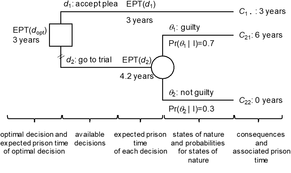
In decision trees, the above decision-theoretic elements are captured as shown in Figure 1. The actions available to the defendant, $d_1$ and $d_2$, are described by the two branches that emanate from the trunk, shown as a square – the decision node – on the far left-hand side. The circled node, also called chance node, represents states of nature about which the decision-maker is uncertain. There is a time order when going from left to right, because when deciding $d_2$, two things can happen. Either, the fact-finder will find the defendant guilty, $\theta_1$, an event thought to occur with probability 0.7, or $\theta_2$, the event of finding the defendant not guilty, an event thought to occur with probability 0.3. At the far right-hand side, the terminal states $C$ are shown, along with their associated evaluation of undesirability (in the case here losses in terms of years of imprisonment). The chance node is labelled with the expected prison term, EPT, of the decision $d_2$ whereas the squared decision node is labelled with the expected prison term of the optimal decision $d_{opt}$. In the analysis here, it is considered that the optimal decision is the one which has the smallest EPT. For the case studied here, the EPT associated with the decision to go to trial ($d_2$), is 4.2, and is obtained by summing over the possible states of nature the product of the loss associated to each consequence $C_{ij}$ (i.e., the prison time ${PT(C}_{ij})$) and the probability of the state of nature, that is:
$${EPT(d}_2)=PT\left(C_{ij}\right)\Pr{\left(\theta_1\middle|\ I\right)}+PT\left(C_{22}\right)\Pr{\left(\theta_2\middle|\ I\right)=6\times0.7+0\times0.3=4.2.}$$
The branch $d_1$ has a smaller EPT, 3 years, which corresponds to the loss associated to the consequence $C_{1\bullet}$, the reduced charge. In summary, thus ${EPT(d}_1)<EPT(d_2)$ and it follows that the optimal decision is $d_{opt}=d_1$.[13] This is in agreement with the assumption that the defence pursues the hypothetical objective of minimizing the expected length of time the defendant will be deprived of liberty. To some extent this helps illustrate why many defendants accept guilty pleas even though they may assign only a moderate or low probability of being convicted if the case went to trial: because the sentence in case of a conviction may be very severe (or perceived as such), even a low probability for a conviction will be sufficient to “outweigh” the sentence associated with the guilty plea. While this is a purely formal view, we concede that in practice defendants may prefer a guilty plea for other reasons, too.
Let us emphasise again that evaluating the undesirability of decision consequences directly in terms of prison time was a choice made for the sole purpose of providing an example, and that other loss functions associating a higher severity to adverse outcomes can be built. This may lead to losses expressing nearly infinitely undesirable consequences that would make going to trial unadvisable even in presence of a very low probability of an unfavourable verdict.[14] Moreover, going to trial may be perceived as a highly aleatory undertaking, with sentence length and probabilities for verdicts being difficult to assess, thus making the guilty plea with its sure consequence the preferable option. Specifically, if the defendant refuses to quantify uncertainty (about states of nature; here verdicts), or refuses to run the risk of incurring the worst consequence associated with going to trial (especially if $C_{21}$ represents a severe sentence), and hence accept the guilty plea ($d_1$), such a strategy would amount to minimising the maximum loss. This is a non-probabilistic decision criterion also known in literature as minimax.[15] It is important to note that such an alternative consideration is not in conflict with the general decision theoretic approach considered here: the basic decomposition of the decision problem outlined at the beginning of this section, summarised graphically in Figure 1, remains the same.
The point of view of the prosecution may be different in that they may seek to maximise the expected prison time, and hence the expected length of time the offender is kept away from society. But again, we emphasise that there may be other – concurrent – objectives in prosecution decision-making, beyond the scope of the generic introductory example chosen here. Our current demonstration only focuses on a single objective and how this single objective is conceptualised. The reader may use other values for probabilities and losses (e.g., different sentence lengths) as required, but should be aware of the fact that this may impact on the EPT of the two decisions, and hence $d_{opt}$. For example, for any plea of guilty on a reduced charge greater than 4.2 years, while keeping the other assignments as defined above, the optimal decision is $d_{opt}=d_2$.
2.2 Bayesian decision networks (influence diagrams)
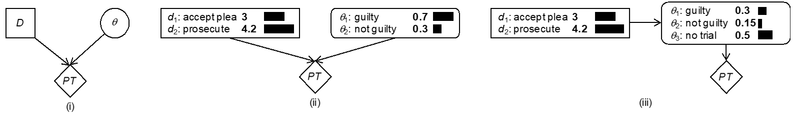
While decision trees (Section 2.1) provide a static summary of the main features of a decision analysis, such as probabilities and (expected) utilities, Bayesian decision networks (BDNs) provide a more flexible and dynamic, but also more compact modelling framework. BDNs extend Bayesian networks by including rectangle nodes for representing decision variables and diamonds for representing utility functions.[16] To illustrate the main components of BDNs, consider again the defendant’s decision problem introduced in Section 2.1. Figure 2 represents the main aspects of this case in terms of a BDN. Rather than presenting a full and simultaneous display of all “routes” that may follow from a decision (as shown in Figure 1), variables in a BDN are represented by single nodes. For example, instead of having a branch for each decision $d_i$ in a decision tree, a BDN concentrates all decisions in a single node (here node D). The expanded node D in Figure 2(ii) summarises the EPT associated with each decision $d_i$. These EPT values correspond to the values attached to the branches $d_i$ of the decision tree (Figure 1). Note that the BDN in Figure 2 is the simplest possible model structure as it involves exactly one node for each node category, i.e. nodes for states of nature (also called chance nodes), decisions and utilities. More elaborate models will be introduced in later sections. Note that the links pointing from nodes D and $\theta$ to PT mean that the “goodness” of a decision, here decision $d_2$, is dependent on the future state of nature $\theta$ (i.e., the trial outcome). In particular, the node PT contains a table that specifies a prison term (in years) for each combination of a decision $d_i$ and a trial outcome $\theta_j$, for $i,j = {1,2}$.
Bayesian decision networks are fairly flexible, as is illustrated by Figure 2 (iii), which shows an alternative network structure. In this model, the states of nature $\theta_j$ depend on the decisions $d_i$. In particular, there is an additional state of nature $\theta_3$, ‘no trial’, that is the situation in which $d_1$ (accept plea agreement) is chosen. The structural relationship $D\rightarrow\theta$ thus allows us to specify probabilities that depend on propositions, $Pr(\theta_j|d_i)$. So, for the case in which the defendant accepts the plea ($d_1$), the conditional probabilities for the states of nature $\theta_j$ are $Pr\left(\theta_j\middle|\ d_1\right)={0,0,1}$, where $\theta_1$=guilty, $\theta_2$=not guilty and $\theta_3$=no trial. And, clearly, if the decision is to prosecute ($d_2$), the probabilities are $Pr\left(\theta_j\middle|\ d_2\right)={0.7,0.3,0}$, for $j = {1, 2, 3}$. The utility node[17] PT contains the values (prison terms) 6 if $\theta_1$ (guilty) holds, 0 if $\theta_2$ (not guilty) holds and 3 if $\theta_3$ (no trial) holds. Note that the latter assignment, ${PT(C}_{1\bullet})=3$, corresponds to the reduced charge associated with the accepted plea.
3 Normative decision structures
3.1 Standard model of legal negotiations
Consider now a standard model of legal negotiations through the case of a hypothetical damage suit in the amount of € 150,000. The plaintiff faces the decision of whether to accept an out-of-court settlement (decision $d_1$), or to bring the lawsuit to trial (decision $d_2$). The plaintiff can either win the case ($\theta_1$), or lose the case ($\theta_2$). Suppose that the plaintiff’s current assessment of his probability of winning the case is 0.8.[18] Using notation introduced above, we can write this as ${Pr(\theta}_1\left|I\right)=0.8$, where I denotes the plaintiff’s current state of information. By coherence, the probability of losing the case is ${Pr(\theta}_2\left|I\right)=0.2$, again considered from the plaintiff’s point of view. Note that in this case the probabilities of states of nature are not conditioned on decisions. For the time being, we will leave aside considerations of litigation costs; we will introduce these step by step later on. The purpose at this point is to draw the attention solely to the notion of the expected value of going to trial, to embody the essence of the problem. In the case here, we suppose that the consequence of a decision is entirely described in monetary terms (monetary value, MV), and that the utility function is linear so that the utility can be set to be numerically equal to the monetary value, that is ${U(MV(d_i,\theta}_j))={MV(d_i,\theta}_j)$. Moreover, we suppose that the decision-maker is willing to act on the basis of expected monetary value (EMV), or at least is interested in this value prior to making a decision based on considerations going beyond those explicitly taken into account at this juncture. As in the previous sections, we emphasise that action based on EMV is an assumption subject to discussion, though it does not impact on the principle of the proposed analyses. It is perfectly feasible, for example, to choose another utility function to account for individual preferences according to which changes in the utility of very low or very high monetary values are not linear.
In the above framework, the optimal decision $d_{opt}$ will be the one at which the EMV attains its maximum, that is
$${EMV(d}_{opt})=\underset{i}{\max}EMV(d_i).$$
We can write the EMV associated with going to trial, for the plaintiff, as follows:
$$\begin{align}{EMV(d}_2)&={MV(d_2,\theta}_1)\times\ {Pr(\theta}_1\left|I\right)+{MV(d_2,\theta}_2)\times\ {Pr(\theta}_2\left|I\right)\newline&= € 150,000×0.8 + € 0×0.2 = € 120,000.\end{align}\tag*{(1)}$$
Note that when deciding $d_1$, there will be no trial, and the plaintiff accepts the out-of-court settlement as given by the monetary value $x$. It is not necessary at this point, to be explicit about $x$. It suffices to note that ${EMV(d}_1)=x$ and the plaintiff will decide $d_1$ whenever ${EMV(d}_1)>{EMV(d}_2)$, that is the settlement offer $x>€ 120,000$. In other words, the plaintiff will decide to go to trial if the expected monetary output, that is the target amount of € 150,000, discounted by probability, is greater than the sure return $x$ from the out-of-court settlement.
3.2 Influence diagrams for the standard model of legal negotiations
In a more realistic perspective, the MV introduced in Section 3.1 should account for the cost of litigation ${l=L(d}_i,\theta_j)$, taken here as the cost incurred by legal representation. Other specific costs may be included in the analysis without loss of generality. Under the reasonable assumption of additivity, since costs are quantified in monetary terms, the monetary value MV can be taken as the net amount which the decision-maker will receive, one has
$${MV(d}_i,\theta_j,l)={MV(d_i,\theta}_j)-L(d_i,\theta_j).\tag*{(2)}$$
The expected monetary value of decision $d_1$ will become
$$\begin{align}{EMV(d}_2)&={MV(d_2,\theta}_1,l)\times\ {\Pr(\theta}_1\left|I\right)+{MV(d_2,\theta}_2,l)\times\ {\Pr(\theta}_2\left|I\right)\newline& =\sum_{j=1}^2[{MV(d_2,\theta}_j)-{L(d_2,\theta}_j)]\times\ {\Pr(\theta}_j\left|I\right).\tag*{(3)}\end{align}$$
In some circumstances, the cost of litigation can be assumed to be independent on the outcome of the trial, that is $L\left(d_2,\theta_1\right)=L\left(d_2,\theta_2\right)=L(d_2)$. Under this assumption, expression (2) can be simplified as
$${MV(d}_i,\theta_j,l)={MV(d_i,\theta}_j)-L(d_i). \tag*{(4)}$$
Litigation costs will then combine naturally with the EMV by subtraction,[19] that is:
$$\begin{align}{EMV(d}_2)&={[MV(d_2,\theta}_1)-L(d_2)]× {\Pr(\theta}_1\left|I\right)+[{MV(d_2,\theta}_2)-L(d_2)]\times\ {\Pr(\theta}_2\left|I\right)
\newline&= \sum_{j=1}^{2}{{MV(d_2,\theta}_j)}\times\ {\Pr(\theta}_j\left|I\right)-L\left(d_2\right).\tag*{(5)}\end{align}$$
In the remainder of this paper, it will be assumed that litigation costs are independent of the outcome of the trial. It is possible, however, to avoid this assumption and adapt the proposed BDNs accordingly as explained later in this section.
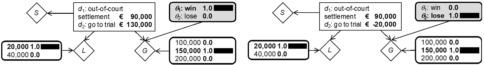
One way to translate the current analysis into an influence diagram consists in reusing the structure of the BDN shown in Figure 2(i) and to change the definition of the nodes D and $\theta$ according to the elements of interest here, i.e. decisions $d_1$ (out-of-court settlement) and $d_2$ (pursue litigation), and states of nature $\theta_1$ (win trial) and $\theta_2$ (lose trial). Note also that the definition of the utility node, denoted G here, shorthand for “gain” understood in a broad sense as defined below, has changed. The resulting model is shown in Figure 3(i). Note that the node G contains the utility function expressed as before in terms of net monetary values: ${MV(d}_2,\theta_1,l)=\ € 150,000-€ 20,000=€ 130,000$, that is the “gain” of winning the trial minus the litigation cost, ${MV(d}_2,\theta_2,l)=\ -\ € 20,000$, i.e. no “gain” when losing the case and incurring the litigation cost, and ${MV(d}_1)=\ € x$, i.e. the offered out-of-court settlement. For the purpose of the current discussion, let $x$ be € 90,000. Note also that when $d_1$ is selected, there is no consideration of the variable $\theta$, the outcome of trial. The EMV of going to trial for the plaintiff’s perspective thus is:
$${EMV(d}_2)=€ 150,000×0.8+€ 0×0.2-€ 20,000=€ 100,000. \tag*{(6)}$$
So, ${EMV(d}_2)>{EMV(d}_1)$ and the plaintiff would refuse the out-of-court settlement in the amount of € 90,000. Note that we do not deal here with the psychological dimension of the decision, in particular the fact that people may be inclined to prefer an out-of-court settlement of € 90,000 that is certain (decision $d_1$) rather than opt for $d_2$ which involves a probability of 0.2 to incur the litigation cost of € 20,000 only, and hence represent a net loss. This would require a different utility function to properly measure the undesirability of a net loss.
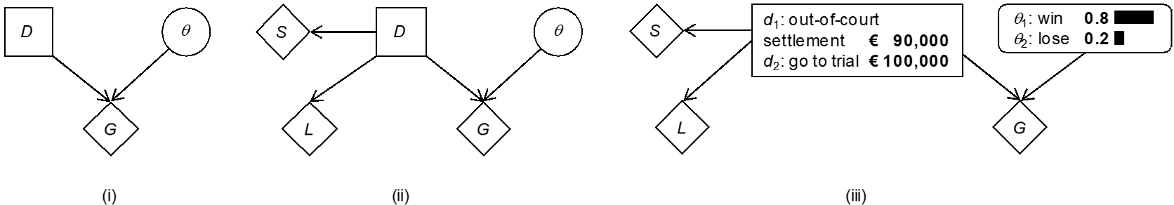
Although being a compact model, Figure 3(i) may be impractical because the monetary values specified in the node G fuse different aspects of the problem, such as litigation costs and gain in case of succeeding at trial. To enhance clarity and exert better control over the different features, it is possible to introduce distinct utility nodes for each monetary factor. This is shown in the BDN in Figure 3(ii) where the node D has child nodes L for the cost of litigation, and S for the out-of-court settlement offer. In this model, the table of the node L specifies – € 20,000 in the event of deciding $d_2$ (pursuing the damage suit at trial). A value of € 0 is specified in the event of $d_1$, not going to trial, because it is assumed that this decision will incur no further litigation costs. A value different from 0 may be chosen, however, to account for costs of option $d_1$ other than legal fees, if required. Specifying the BDN in this way using, for example, a Bayesian network software such as HUGIN,[20] leads to model output shown in expanded version in Figure 3(iii).[21] The decision node displays the EMV of the options $d_1$ and $d_2$, and the chance node $\theta$ shows the plaintiff’s probabilities for the trial outcomes $\theta_1$ and $\theta_2$. It may be argued that none of these results are original, because they may also be obtained using paper and pencil. It is relevant, however, to pursue the development of these models stepwise, starting with simple formats, in order to lay bare their constructional logic and demonstrate that their output can be trusted. This represents an important preliminary step to more advanced network structures for which the underlying calculations, without computational support, become increasingly complex. The next section illustrates the ease with which further features can be added.
3.3 Uncertainty about verdicts and litigation costs
A restriction of the models introduced so far is that factors such as the amount in case of winning at trial (e.g., node G, Figure 3) and litigation costs are considered fixed or known monetary values. However, at the time of making a decision, the plaintiff may be uncertain about the length of the process and the court-ordered settlement (i.e., the amount granted in case of a verdict favourable to the plaintiff). We now point out how BDNs can readily handle such additional sources of uncertainty.
Start by considering uncertainty about the litigation costs. These may crucially depend, for example, on process length and case complexity. For the purpose of illustration, suppose that the plaintiff considers that – given consideration of the case as a whole – it is more probable than not that litigation costs will be twice as high, that is € 40,000, rather than € 20,000 as in the previous section. How does this affect the EMV of the decision $d_2$ of going to trial? Let us assume that the plaintiff wishes to consider two different cases, i.e. litigation costs of € 20,000 with probability 0.4, and € 40,000 with probability 0.6. The reader may consider other amounts and associated probabilities. The expected cost of litigation thus is: $€ 20,000×0.4+€ 40,000×0.6=€ 32,000$. Using this result in Equation (5), the EMV of going to trial for the plaintiff’s perspective thus becomes:
$${EMV(d}_2)=€ 150,000×0.8+€ 0×0.2-€ 32,000=€ 88,000. \tag*{(7)}$$
Since the expected cost has increased by € 12,000, the EMV of decision $d_2$ has decreased by the same amount. In particular, note that now ${EMV(d}_2)<\ {EMV(d}_1)$ so that the out-of-court settlement € 90,000 becomes more advantageous – it becomes the optimal decision – for the plaintiff, although the plaintiff may consider this difference to be rather small. The proposed BDN can be further developed to acknowledge for more realistic settlements where the cost of litigation is a function of the process length. For example, one may consider the litigation cost to be proportional to the fee per hour of a lawyer, by adding a node to acknowledge for the expected length of the trial.
Next, consider uncertainty about the amount granted in case of a verdict favourable to the plaintiff. Assume, for example, that the party considers three possible amounts granted or court verdicts, € 100,000, € 150,000 and € 200,000, with associated probabilities 0.3, 0.6 and 0.1. Thus, the fixed ${MV(d}_2,\theta_1)$ in Equation (5) must be replaced by the expected monetary value, that is the sum of the three outcomes weighted by their probability, that is $€ 100,000×0.3+€ 150,000×0.6+€ 200,000×0.1=€ 140,000$. Inserting this result in Equation (5) gives:
$${EMV(d}_2)=€ 140,000×0.8+(€ 0)×0.2-(€ 32,000)=€ 80,000. \tag*{(8)}$$
Thus, uncertainty about the amount of the court-ordered settlement has led to a further decrease of the EMV, in addition to that incurred by uncertainty about legal fees, so that there is now a more clear-cut difference with respect to the EMV of $d_1$, which is given by the out-of-court settlement amount of € 90,000.
To track the above results in a BDN, consider an extension of the model in Figure 3(ii), shown here in Figure 4. This network contains an additional node L′ with two states 40,000 and 60,000 to which unconditional probabilities 0.4 and 0.6 are assigned. This node models the different litigation costs and the plaintiff’s probabilities for these costs in case decision $d_2$ is made. Adding node L′ as a parent for L requires a modification of the node table of L so that it will copy the negative value[22] of the current state of L′ when the condition ${D=d}_2$ holds, and the value 0 otherwise. Software environments such as Hugin offer a rich syntax (e.g., if-then expressions) to define functions in this way. Similarly, there is an additional node G′, acting as a parent node for G. The states of G′ correspond to the different court-ordered settlements, whereas the associated node probability table contains the plaintiff’s probabilities for those outcomes in the event decision $d_2$ is made. The node table of G is defined[23] such that it copies the current value of G′ in the case where both ${D=d}_2$ and $\theta_1$ holds, and the value 0 otherwise.
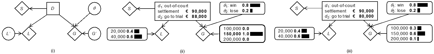
Figure 4(ii) shows a schematic illustration of the compiled network. The node G′ is fixed (i.e., instantiated) to the state € 150,000, highlighted with a bold border line. This corresponds to a situation in which there is no uncertainty about the court-ordered verdict. In turn, the node L′ is left uninstantiated so as to allow for uncertainty about the litigation costs. For such a situation, the node D shows that the EMV of decision $d_2$ is € 88,000, which corresponds to the value found through Equation (7). The network shown in Figure 4(iii) shows a situation that allows for uncertainty about the court-ordered settlement, which is achieved by leaving the node G′ uninstantiated. The EMV of decision $d_2$ then is € 80,000, which corresponds to the result given by Equation (8).
3.4 The notion of perfect information (PI)
The previous sections have illustrated that the major factor rendering decision-making hard is uncertainty about the state of nature $\theta$, for if we knew whether $\theta_1$ (win) or $\theta_2$ (lose) holds, choosing between $d_1$ and $d_2$ is more straightforward. In the special case where other factors (e.g., litigation costs) could be considered fixed (i.e., without uncertainty), it would even be possible to tell which decision would offer the most desirable outcome within the stated modelling assumptions. Therefore, any information capable of reducing uncertainties about the states of nature, that is directing associated probabilities towards $0$ and $1$, is of particular interest to decision-makers. One notion that is often encountered in this context is perfect information (PI). This represents an element that is completely informative about the propositions of interest (i.e., information that would allow one to know which proposition is true). A crucial question is, however, how valuable such data or information is. This question is pursued below. Although it may be considered a hypothetical question, it is useful as a starting point for thinking about the more general issue of data that are only partially informative (i.e., imperfect). Such data do not allow us to establish with complete certainty which state of nature actually holds, a property that typically applies to forensic science results.
Perfect information can lead to two different outcomes. In one case, perfect information would establish $\theta_1$, i.e. winning the case. The best decision then is $d_2$, pursuing the dispute, because the outcome will be a verdict of € 150,000, from which the litigation costs of € 20,000 must be subtracted. The second possibility is that perfect information establishes $\theta_2$, in which case decision $d_2$ would incur the litigation costs of € 20,000, and no “gain”, whereas $d_1$ would lead to the out-of-court settlement of € 90,000 (a situation in which no litigation cost is assumed). But again, the states of nature are unknown, so at best one can consider one’s expected outcome (monetary value) with perfect information (EMVPI), defined as follows:
$$EMVPI=\sum_{j=1}^2[\underset{i}{\max}({MV(d_i,\theta}_j) – L(d_i))]\times\ {\Pr(\theta}_j\left|I\right). \tag*{(9)}$$
In the example considered here, this results in $€ 90,000-€ 20,000×0.8+€ 90,000×0.2=€ 122,000$. Stated otherwise, the expected outcome with perfect information is obtained by summing over the possible states of nature (or outcomes) the maximum net monetary value – that is the monetary outcome associated with the optimal decision – weighted by the probability of the state of nature.[24]
The EMVPI can be compared to the EMV of the optimal decision without perfect information. For a case in which the verdict is taken to be constant at € 150,000, and the litigation cost fixed to € 20,000, the decision $d_2$ was found to be optimal, with an EMV of € 100,000, found through Equation (6) and also shown in Figure 3(iii). The result of this comparison is the expected value of perfect information (EVPI), that is € 22,000. It is often referred to as the maximum price that one should be willing to pay for obtaining such perfect information. More formally, it is defined as follows:
$$EVPI=EMVPI{-EMV(d}_{opt}).\tag*{(10)}$$
where dopt is the optimal decision without additional information, also sometimes called the a priori optimal action.
The EVPI does not correspond to a particular state of a BDN, and hence cannot directly be read off the graph.[25] Rather, Equation (10) shows that the EVPI is the result of a comparison of different situations, and those can be displayed separately. As is illustrated by Figure 5, for example, one can determine the optimal decisions and their associated EMVs under assumptions of perfect information, which is needed to calculate the EMVPI, as part of the EVPI. The added value of BDNs thus is to provide a unified environment in which one can break down abstract formulae, such as Equation (9), into their constituting components, which may otherwise be more difficult to achieve, and more prone to error.
3.5 Expected value of partial information (pI)
In legal practice, it is often the case that a party has the option of seeking further evidence that may have a bearing on the assessment of probabilities for trial outcomes. Typically, information that may be gathered in real cases is not such as to establish clear-cut values of $0$ and $1$ for the probabilities of the states of nature as is supposed by perfect information (Section 3.4). Let us denote such evidence partial information (pI).[26] To assess the expected value of less than perfect information, one needs to consider the effect that partial information has on one’s probabilities for the relevant states of nature $\theta$. Given the probabilistic graphical modelling framework used in this paper, this operation is naturally operated through Bayes’ theorem.[27] The procedure is outlined below. A forensic example is given in Section 3.6.
Consider first that the optimal decision d with partial information E, say $d_{opt|E}$, is the one that maximises the EMV calculated on the basis of the posterior probabilities for the trial outcomes $\theta$ once the partial information E is available, say $Pr(\theta|E)$. Formally, thus, $d_{opt|E}$ is the decision at which the EMV attains its maximum:
$$\begin{align}{EMV(d}_{opt|E})&=\underset{i}{\max}{EMV\left(d_i\middle|E\right)}
\newline&=\underset{i}{\max}\sum_{j=1}^2[{MV(d_i,\theta}_j) – L(d_i)]\times\ {\Pr(\theta}_j\left|E\right).\tag*{(11)}\end{align}$$
For shortness of notation only, we leave aside relevant information I from notation and assume that there are fixed monetary values for the trial verdict in case of winning, that is ${MV(d}_2,\theta_1)$, and the litigation costs ${L(d}_2)$. Also, the out-of-court settlement has a fixed value ${MV(d}_1)$, which is independent of \theta, with no associated litigation cost.
Equation (11) provides the guide to action in case the decision-maker knows what kind of information E has been obtained, and hence posterior probabilities $Pr(\theta_j|E)$ are available. However, information E may take various different forms (i.e., $E_k$, for $k=1,2,…,n$), so that prior to obtaining E the decision-maker should take into account these possible outcomes $E_k$, along with an expression of the associated uncertainty, in terms of probabilities. This leads to the expected monetary value with partial information (EMVpI):
$$EMVpI=\sum_{E}\underset{i}{\max}{EMV\left(d_i\middle|E\right)\times\ Pr(E)\tag*{(12)}}$$
Equation (12) involves the multiplication of results in (11) by $Pr(E)$ over the various possible forms that the information E can take.[28] The difference between this result and the EMV without information E is the expected value of partial information (EVpI):
$$EVpI=EMVpI-\underset{i}{\max}{EMV(d_i),\tag*{(13)}}$$
where $\underset{i}{\max}{EMV(d_i)}$ is $EMV(d_{opt})$, prior to the partial information E.
3.6 Example: EMV of partial forensic information
To illustrate the consideration of partial information with a forensic connotation, suppose that E refers to the report of a forensic document examiner. Forensic document examinations focus on a variety of aspects, such as physical document examinations or comparative handwriting examinations. The results of such examinations may help inform about document authenticity, for example, which may be a key issue in a litigation case. Assume that the conclusion of the report of the forensic scientists takes one of the following three different forms: findings (i.e., evidence) favourable to the plaintiff ($E_1$), neutral findings (i.e., favouring neither party; $E_2$), and findings favourable to the defendant ($E_3$). Note that this is a general way of looking at the forensic scientist’s work, comparable to that of other specialists and consultants that may be contacted as part of the legal process.
What exactly forensic and other specialists are consulted for is a crucial point that is worthy to be defined in more detail. In particular, we emphasize that the issue here is not the use of results of forensic examinations to help inform about intermediate propositions such as “the questioned document was signed by the defendant” versus “an unknown person signed the questioned document”, or “the questioned document was printed with the defendant’s device” versus “an unknown printer was used”. Such propositions are used in conventional evaluations of forensic results.[29] Here a different uncertain proposition is of interest: it is the outcome of the lawsuit, denoted $\theta$, which is the uncertain event bearing on the decision analysis.[30]
The decision analyst thus is directed to think about how the forensic report E informs the party about $\theta$, the verdict at the end of the trial. Let us emphasise again that the question here is not one of weight of evidence for results of forensic examinations, a notion concerned with propositions representing competing versions of an event of interest. The focus here is the impact on verdicts, i.e. how a given forensic conclusion will impact, as judged by the litigant, the relative probabilities of the two possible ultimate trial outcomes. In a formal framework, a logical way to track this question is through Bayes’ theorem. With the prior probabilities $Pr(\theta)$, obtaining the posterior probabilities $Pr(\theta|E)$ requires the consideration of the probabilities for E given $\theta$, $Pr(E|\theta)$. Suppose the following values: ${Pr(E}_i\left|\theta_1\right)={0.9,0.05,0.05}$ and ${Pr(E}_i\left|\theta_2\right)={0.1,0.05,0.85}, for\ i = 1, 2, 3$. These assignments express the view that a forensic finding favourable to the plaintiff ($E_1$) is more probable if the case in fact turns out favourably for the plaintiff ($\theta_1$), rather than unfavourably ($\theta_2$). The assignment also conveys the view that a result unfavourable for the plaintiff ($E_3$) is more probable if the case in fact turns out unfavourably for the plaintiff ($\theta_2$), rather than favourably. It is also considered that a “neutral” forensic result ($E_2$) is obtained with the same probability under each state of nature $\theta$. Note that these probabilities are also sometimes interpreted as a consideration of an expert’s reliability. This is comparable to other contexts where, for example, expert evidence is used to inform about states of nature such as the presence or absence of oil or gas on a potential mining site, or the commercial success of a new product introduced on the market.
Clearly, finding the EVpI through Equation (13) with the above assignments is a tedious task. However, we can illustrate the support provided by computationally implemented Bayesian decision networks. They can either break down the computation into smaller chunks or even provide the result in a single step. The latter may be preferable if efficiency is required, whereas the former may be of interest if intermediate results (e.g., the optimal decision and associated EMV for a given result E) need to be inspected. This may be valuable when consulting with a client because it will allow the analyst to work through the decision network together with the client to demonstrate how the optimal decision may change in different circumstances, and that the analyst has seriously assessed each aspect of the client’s case. Below, we briefly outline both routes.
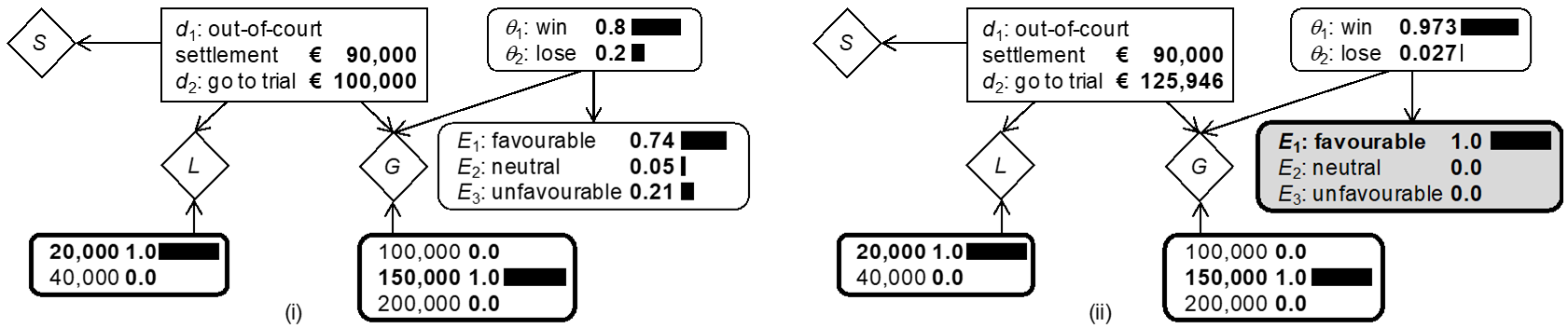
Start by considering the computation of parts of the EVpI using the BDN shown in Figure 6(i). It contains an additional chance node for the possible forensic findings E, specified as a child node of $\theta$ (trial outcome). The conditional probabilities $Pr(E|\theta)$ are as assigned above. Figure 6(i) shows the BDN in its initial state, with nodes G′ and L′ fixed to, respectively, € 20K and € 150K. The node E shows the marginal probabilities for the various forms that the forensic report may take. These values are one element needed for the EMVpI (Equation (12). Further elements are posterior probabilities for $\theta$ and the EMV of the optimal decision given a particular posterior probability distribution over $\theta$.[31] This is illustrated in Figure 6(ii) for the situation in which the outcome $E_1$, a favourable forensic report (for the plaintiff’s position), is obtained: it is shown that the posterior probability ${Pr(\theta}_1|E_1)$ increases to 0.973 and the optimal decision is $d_2$, with an EMV of € 125,946. One can proceed analogously for the potential outcomes $E_2$ (neutral forensic report) and $E_3$ (unfavourable forensic report). Applying the results in Equation (12) leads to the EMVpI of € 117,100. Comparing this result with the EMV € 100K of the optimal decision without partial information, shown in Figure 6(i), gives the EVpI of € 17,100. For a summary of the computation of the EMVpI, see also Table 1. Note that this listing of the various outcomes and the optimal decisions in each of these cases is also sometimes referred to as a policy.
| Forensic result E | ${\Pr(\theta}_1\left|E_i\right)$ | $d_{opt|E}$ | ${EMV(d}_{opt|E})$ | ${EMV(d}_{opt|E})\times Pr(E)$ |
| $E_1$ (favourable) | {0.973,0.027} | $d_2$ | € 125,946 | € 93,200 |
| $E_2$ (neutral) | {0.8,0.2} | $d_2$ | € 100,000 | € 5,000 |
| $E_3$ (unfavourable) | {0.19,0.81} | $d_1$ | € 90,000 | € 18,900 |
| Total: € 117,100 | ||||
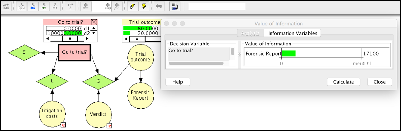
The direct computational step to obtain the EVpI for the forensic report E is shown in Figure 7, using the “Value of information” functionality of the software Hugin. The EVpI can be retrieved in an information pane while keeping track of other key values shown in monitor windows besides nodes in the network (e.g., EMV of the a priori optimal action, here $d_2$, which is € 100K).
3.7 Sequential decision-making and normative decision policies
So far we have considered a formal way of thinking about the value of a single item of information in the context of making an important decision, illustrated through the example of a hypothetical litigation case. This analysis can be taken a step further and be reflected on from the perspective of sequential decision-making. In the currently discussed example, the decision about whether or not to obtain forensic information is made before making a decision about bringing the damage suit to trial. Thus, there is a sequence of decisions. In terms of a Bayesian decision network, the decision about obtaining or not forensic information can be represented by adding an additional decision node, denoted F here, as a parent for the node E. The values of the node F are “acquire forensic information ($f_1$)” and “do not acquire forensic information ($f_2$)”. The node F has a utility node K as a child, in order to account for the cost of the forensic information. The chance node K′ deals with uncertainty about these costs as done previously for the nodes G′ and L′. Figure 8 summarises the network. Note that there are additional edges with dotted lines. One edge is a precedence link and goes from the decision node F to the decision node D. This indicates the temporal order that decision F precedes decision D. Another edge, an information link, goes from E to D. This dotted edge indicates that the state of the variable E is known before the ultimate decision D is made. These semantic aspects are also known as the no-forgetting assumption: the decision-maker perfectly recalls all “experiments” and decisions made in the past.
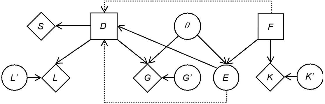
The definition of the node E has slightly been changed, by adding a further state called “no result”. It accounts for the situation in which the node F takes the value “do not acquire forensic information ($f_2$)”. The definition of the conditional probability table for the node E from Section 3.6 is modified to $Pr\left(E_i\middle|\theta_1,F=f_1\right)=\{0.9,0.05,0.05,0\}$ and $Pr\left(E_i\middle|\theta_2,F=f_1\right)=\{0.1,0.05,0.85,0\}, for\ i = 1,2,3,4$. In case of ${F=f}_2$, not acquiring forensic information, we specify $Pr\left(E_i\middle|\ F=f_2\right)=\{0,0,0,1\}$, regardless of the state of the node $\theta$.
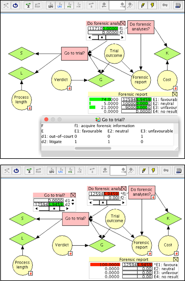
Implementing the Bayesian decision network shown in Figure 8 in a graphical modelling software, such as Hugin, allows one to conduct a variety of analyses. A first important question is: “Should forensic information be acquired?”. To answer this question, we need the ${EMV(f}_1)$. In Hugin, this value can be obtained by using the iterative algorithm called “Single Policy Update”. As shown in Figure 9 (top), the value obtained is 117,000, which corresponds to the EMVpI found at the end of Section 3.6 (see also Table 1). This value is greater than the EMV 100,000 for not conducting forensic analyses (not shown in Figure 9). Note that the cost for the forensic analyses has been set to zero here in order to allow for a direct comparison of the output with the results obtained in Section 3.6.
Following the decision to acquire forensic analyses (decision node F), the next question will be whether or not to bring the case to trial (decision D). This second decision is considered here to depend on the outcome of the forensic report. To help with this question, consider again Figure 9 (top). The monitor window of the node E (“Forensic report”) shows the probabilities for obtaining the various reports outcomes $E_i, for\ i = 1, …, 4$, as well as the EMV of the optimal terminal decision at the node D (“Go to trial?”). As may be seen, these values correspond to the ${EMV(d}_{opt})$ obtained in column 4 of Table 1. Note, however, that the optimal decisions $d_{opt}$ vary: for a favourable ($E_1$) and a neutral ($E_2$) report, the optimal decision is $d_2$ (go to trial); for an unfavourable report ($E_3$), the optimal decision is $d_1$, accepting the out-of-court settlement offer. The EMV of the latter decision can readily recognised to be 90,000, as defined in Section 3.2. The optimal decisions for the node D (“Go to trial?”) given each outcome $E_i$ are summarised in a so-called policy table, as shown at the bottom of Figure 9 (top). This table contains the value 1 for the optimal decision, and 0 otherwise. Figure 9 (bottom) illustrates the state of the network after obtaining a favourable forensic report and communicating this information to the network. The optimal decision in such a situation is to bring the case to trial, decision $d_2$, with EMV 125,946.
A particular feature of the semantics of the Bayesian decision network considered here is the notion of “decision past”. A decision node in a Bayesian decision network has a decision past that includes the parents of the decision node of interest, as well as the previous decisions in the decision sequence with their parents. A policy for a decision node in a Bayesian decision network specifies a decision for any possible configuration of the decision past of the decision node of interest. Here, a configuration means a possible combination of decisions and observations made prior to making the decision of interest. In Table 2 we specify different decision pasts for the node D (“Go to trial?”), and associated policies. We refer to them as normative decision policies.
| Do forensic analyses? | Forensic report | $EMV(d_1|E_i)$ | $EMV(d_2|E_i)$ | Optimal decision |
| yes | $E_1$: favourable | 90,000 | 125,946 | $d_2$: go to trial |
| yes | $E_2$: neutral | 90,000 | 100,000 | $d_2$: go to trial |
| yes | $E_3$: unfavourable | 90,000 | 8,571 | $d_1$: settle |
| no | $E_4$: no result | 90,000 | 100,000 | $d_2$: go to trial |
4 Discussion and conclusions
Traditionally, scholarly literature on how to manage information in the legal process has largely gravitated around questions of probative value of the evidence in the case at hand. In particular, it has focused on whether and to what extent evidence has discriminative capacity with respect to the competing propositions presented by the parties at trial, and how evidence impacts the ultimate issue on which factfinders need to render a decision. However, this emphasis on the fact-finders’ perspective is only a small part of the broad scope of weight-of-evidence and decision-making issues that the various participants in the legal process encounter. For example, litigants may need to decide whether or not to go to trial, and whether or not to look for additional information before taking further legal action. Most often, such questions are thought about and formulated in a verbal and qualitative way; this is often felt to be insufficient because of the high stakes involved, which can be quantified to at least some extent (e.g., in monetary terms). Costs for legal representation and ongoing enquiries raise questions such as “how much should we be willing to pay for additional information?” or “what is the (expected) value of additional information?”. The legal context in which such questions are raised being highly complex, and information coming in natural language, formal approaches to analysing case-tailored legal strategies are a pending challenge, as demonstrated by the numerous directions that research has taken around the notions of artificial intelligence and legal analytics.[32]
The formal modelling approach presented in this paper aims to cope with the above challenges, though it is important to be clear about a few key characteristics of our analyses.
- First and foremost, the computational models we describe are not autonomous systems. Any decision-analytic model needs to be built for the specific needs of the case at hand, and requires choices to be made by the decision analyst on (i) which variables to include in the analysis (e.g., litigation costs), (ii) the general level of detail at which the decision problem is to be approached (e.g., which uncertainty factors ought to be included) and (iii) assessments of probabilities and utilities. Though generic template structures may be given (e.g., the standard model for legal negotiations, Section 3.1), they need to be adapted to the particular needs of the case of application. Thus, the normative decision structures discussed in this paper are not attempts at replacing decision analysts, but are intended to support analysts in their probabilistic thinking and decision making, using formal theories, at a level of sophistication that may become unfeasible or discouraging without computational support.
- The graphical modelling language and its possibilities for computational implementations are both rigorous and liberal concepts: they are rigorous in the sense that they capture relevance relationships among fundamental elements of decision problems in a logically sound way (i.e., in agreement with principles of probability and decision theory), and they are liberal in that they can cope with various levels of detail at which the analyst is willing to operate.
- The proposed decision analytic structures are normative in that they assert coherence, i.e. conformity with probability and decision-theoretic principles. They are not generally normative, but only with respect to the elements specifically taken into account in the given case and at the level of detail chosen by the analyst. Although the elements included in an analysis are supposed to be those deemed most crucial, we do not consider the normative answers to be prescriptive because litigants may deliberately choose actions that are not considered optimal in the sense understood in the normative analysis. For example, litigants may seek to engage in legal action despite the fact that the monetary prospects of their decisions are not optimal, because it helps them attain other objectives, such as damaging their opponent’s reputation. The role of normative analyses is to provide a point of comparison against which decision-makers can compare their reasoning, prior to actually making a decision, so as to gain a better awareness as to what exactly their choices entail, and compare their (intuitive) choices to the results of formal decision-theoretic analyses.
Criticism is recurrently raised against formal modelling approaches in legal analytics. One critique is levelled at the concept of probability as used in this paper, for example, when assessing a party’s considerations of how a verdict will turn out. Practitioners may dislike the particular numerical form in which the proposed models employ probability, though fundamentally the notion of probability cannot be dissociated from litigants’ case analyses: their considerations necessarily imply an assessment of the prospect of winning a given case.[33] However, there are potential solutions to this problem, as is illustrated, for example, by research efforts into models of “forecasting” (or, “predicting”) legal outcomes.[34] These may assist in providing probabilistic assessments for input values of the decision-theoretic models developed in this paper. Note, however, that such research currently focuses on selected court levels (e.g., U.S. Supreme Court) and requires considerable past data. In any event, an assessment – probabilistic or otherwise – of particular court outcomes is not the end of the matter: once a given assessment for legal outcomes in the case at hand is obtained, the practitioner still has to choose a course of action. This question, as we have argued throughout this paper, requires consideration of the various decision consequences and their relative merit from the litigant’s personal point of view. The decision-theoretic modelling approach presented here have several advantages to capture such thinking. For example, clients may want to obtain from their attorney an assessment that is based on more than just an attorney’s reference to past experience or performance. Using a formal model, attorneys (possibly assisted by decision-analysts familiar with the technicalities of the method) can demonstrate that they have seriously considered the key aspects of a case when suggesting a given course of action. Computationally implemented decision-theoretic models also provide visual support to help clarify the expected outcomes of different litigation strategies. This can be of interest to legal practitioners who seek to ensure that their clients are an integral part of the process of litigation strategy development.
But still, the quantitative assessment of the relative (un-)desirability of decision consequences and the partial nature of decision-theoretic models with respect to the broad complexity of practical decision problems also invite criticism, with regards to practicality. While this is a valid argument, the same problems are even more acute when these challenges are dealt with in an intuitive and formally unaided way. Thus, the computational model structures discussed in this paper contribute to the variety of approaches available to legal practitioners who must constantly assess how they can improve the quality of advice provided to their clients, which is also a critical topic for current legal educational curricula.[35]
Acknowledgments
The research reported in this paper has been supported by the Swiss National Science Foundation through grants No. BSSGI0_155809 (Alex Biedermann) and No. PP00P1_176720 (Joëlle Vuille). Alex Biedermann gratefully acknowledges helpful comments received from members of CodeX (The Stanford Center for Legal Informatics).
[1] E.g., Howard Raiffa, Decision Analysis, Introductory Lectures on Choices under Uncertainty (Reading, Mass.: Addison-Wesley, 1968); Howard Raiffa and Robert Schlaifer, Applied Statistical Decision Theory (Cambridge, Mass.: MIT Press, 1961).
[2] John von Neumann and Oskar Morgenstern, Theory of Games and Economic Behavior, 3rd ed. (Princeton: Princeton University Press, 1953).
[3] Alan Cullison, “Probability Analysis of Judicial Fact-Finding: A Preliminary Outline of the Subjective Approach” (1969) 1 University of Toledo Law Review pp. 538-698; John Kaplan, “Decision Theory and the Factfinding Process” (1968) 20(6) Stanford Law Review 1065-1092.
[4] Stuart Nagel, Microcomputers as Decision Aids in Law Practice (New York: Quorum Books, 1987); Stuart Nagel, Decision-Aiding Software and Legal Decision-Making: A Guide to Skills and Applications Throughout the Law (New York: Quorum Books, 1989).
[5] Ronald Howard, “Decision Analysis and Law” in Marilyn Mac Crimmon and Peter Tillers (eds.), The Dynamics of Judicial Proof. Computation, Logic, and Common Sense (New York: Springer, 2002), pp. 261-269.
[6] E.g., Howard Raiffa, The Art and Science of Negotiation, How to Resolve Conflicts and Get the Best out of Bargaining (Cambridge, Mass.: Belknap Press of Harvard University Press, 1982).
[7] Uffe Kjærulff and Anders Madsen, Bayesian Networks and Influence Diagrams, A Guide to Construction and Analysis (New York: Springer, 2008).
[8] Franco Taroni et al., Bayesian Networks for Probabilistic Inference and Decision Analysis in Forensic Science, 2nd ed., (Chichester: John Wiley & Sons, 2014).
[9] Dennis Lindley, Making Decisions, 2nd ed. (Chichester: John Wiley & Sons, 1985).
[10] Johnathan Baron, Thinking and Deciding (New York: Cambridge University Press, 2008, 4th ed.).
[11] E.g., Terry Connolly, “Decision Theory, Reasonable Doubt, and the Utility of Erroneous Acquittals” (1987) 11(2) Law and Human Behaviour 101-112; Gregory Jones and Douglas Yarn, “Evaluative Dispute Resolution Under Uncertainty: An Empirical Look at Bayes’ Theorem and the Expected Value of Perfect Information” (2003) 2 Journal of Dispute Resolution 427-461; Daniel Kahneman, Thinking, Fast and Slow (London: Penguin, 2011).
[12] In the context of evaluating the impact of evidence, the proposition “the defendant committed the crime” is sometimes referred to, colloquially, as the “guilt hypothesis”. This has been criticised as confusing (e.g., Ronald Allen, “Rationality, Algorithms and Juridical Proof: a Preliminary Inquiry” (1997) 1 The International Journal of Evidence & Proof 254-275; Stephen Fienberg, “Theories of Legal Evidence: What Properties Should They Ideally Possess and when are they Informative?” (1997) 1 The International Journal of Evidence & Proof 309-312) because, strictly speaking, guilt is not a hypothesis, but a decision reached based on the consideration of the proposition according to which the defendant is the offender. We agree with this view. In our decision analysis pursued here, a court’s decision is considered an uncertain state of nature for which a participant in the legal process (e.g., the defendant) may assign probabilities. Hence, we are not modelling the trial decision, but the decision of what to do from the point of view of a participant (party) in the legal process.
[13] The elicitation of probabilities for states of nature is often considered a tedious task, since decision-makers are asked to translate into numbers their personal beliefs, sometimes with an unrealistic level of precision. However, the decision-maker can perform a sensitivity analysis to provide a threshold for the required probability with which the optimal decision will change. In the current example, one may easily observe that the limiting value for is equal to 0.5: as long as the event that the court will find the defendant guilty is considered to be more probable than the event that the court will render a verdict of not guilty, the optimal decision is . The assignment of losses is another intricate task. Clearly, one may observe that the consequence of a conviction, resulting in prison, may not be linear over the total range of years of imprisonment, with a decreasing aversion to prison time. It is possible to build a loss function in the range (0, 1), with a zero loss associated with an acquittal, and a maximum loss equal to 1 in the case of, for example, life imprisonment, with highly increasing losses over the first years, followed by a linear growth. This may obviously have an impact on the optimal decision, though this does not adversely affect the proposed approach as such. The fact that an optimal decision may vary depending on one’s assumptions and preferences does not imply that the implemented decisional approach is unsuitable. A decision, in the approach pursued here, is not optimal in absolute terms; it is optimal with respect to the decision-maker’s preferences and uncertainties about outcomes at stake.
[14] The reason for using the term “nearly infinitely undesirable consequences” is that the axiomatic foundation for the existence of a utility function we refer to requires that there do not exist infinitely undesirable consequences. Otherwise, no matter how small the probability of a conviction is, one will always prefer to avoid going to trial.
[15] E.g., Herman Chernoff and Lincoln Moses, Elementary Decision Theory (New York: John Wiley & Sons, 1959).
[16] Kjærulff and Madsen, supra n. 7.
[17] Note that the “utility” in this case represents, in fact, a loss. However, this has no impact on the optimisation strategy and the resulting decisional choice: the criterion of maximising expected utility will become the criterion of minimising expected prison time (i.e., loss).
[18] How to arrive at such probability assignments is an intricate topic in its own right and goes beyond the scope of this paper. Devices that can help with probability assignment are covered largely in specialised literature on the topic, ranging from practical approaches (e.g., consultation with peers, past experience in similar cases, etc.) to technical procedures based on chance devices (e.g., probability wheels) adapted from fields such as applied psychology (see, e.g., Howell Jackson et al., Analytical Methods for Lawyers (St. Paul, Mn.: Foundation Press, 2003), pp. 27-30; Baron (2010), supra n. 10, pp. 112-113; Detlof von Winterfeldt and Ward Edwards, Decision Analysis and Behavioral Research (Cambridge: Cambridge University Press, 1986), pp. 112-122).
[19] It is important to note that this is valid only under the assumption of linearity of the utility function. In fact, one has . If, however, the utility function is not linear, and the assumption of additivity cannot be made.
[20] https://www.hugin.com; Kjærulff and Madsen, supra n. 7.
[21] Note that Figure 3 contains schematic illustrations, not screenshots of BDN software.
[22] A negative value is specified here because in Hugin utility nodes are considered as additive contributions to the utility function.
[23] In Hugin syntax, an expression such as if(and(D==”d2″,theta==”win”),Gprime,0) may be used, where D, theta and Gprime correspond to the internal names of the nodes D, $\theta$ and G′.
[24] Note that the procedure is general and also holds for n hypotheses.
[25] Note, however, that some graphical probability software packages (e.g., Hugin) offer built-in functions to perform value of information analyses.
[26] Here, the lower-case letter “p” denotes “partial” as compared to the capital letter “P” used to denote “perfect” in Section 3.4.
[27] For the purpose of this paper, it is not necessary to go into the technical details of operating Bayes’ theorem because this is a feature incorporated by default in Bayesian (decision) networks (e.g., Uffe Kjærulff and Anders Madsen (2008), supra n. 7).
[28] Note that the sum in Equation (12) may be replaced by an integral to deal with continuous evidence. In this latter case, the probability of the evidence will be replaced by a probability density.
[29] Colin Aitken and Franco Taroni, Statistics and the Evaluation of Evidence for Forensic Scientists, 2nd ed. (Chichester: John Wiley & Sons, 2004); Franco Taroni et al., Data Analysis in Forensic Science: a Bayesian Decision Perspective (Chichester: John Wiley & Sons, 2010); see also supra n. 12.
[30] It is worth noting, though, that some propositions of interest when evaluating forensic results (e.g., “the questioned signature is authentic”) are closely related to ultimate propositions (e.g., liability).
[31] Again, these probabilities are obtained through Bayes’ theorem (see also supra n. 27).
[32] E.g., Kevin Ashley, Artificial Intelligence and Legal Analytics, New Tools for Law Practice in the Digital Age (Cambridge: Cambridge University, 2017).
[33] For arguments in favour of efforts to elicit numerical probabilities in litigation analysis see, e.g., Marc Victor, “The Proper Use of Decision Analysis to Assist Litigation Strategy” (1985) 40 The Business Lawyer 617–629.
[34] For a recent example and overview see, e.g., Daniel Katz, Michael Bommarito and Josh Blackman, “A General Approach for Predicting the Behavior of the Supreme Court of the United States” (2017) 12(4) PLOS ONE 1-18.
[35] Paul Brest and Linda Krieger, Problem Solving, Decision Making, and Professional Judgment, A Guide for Lawyers and Policy-makers (Oxford: OUP, 2010).